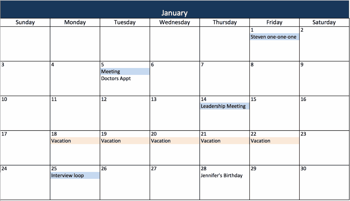
In Microsoft Excel, you can create a dynamic annual calendar using a few simple formulas. This calendar will then automatically adjust to subsequent years when you change the year.
Create a yearly calendar in Excel
To create the Excel annual calendar with just a few formulas, you first need to do some preparation.
- Enter the year in the top row. If you want, you can give your calendar a name in the row below.
- Go down one field and connect three cells there. Use the “Merge and center” setting for this.
- In these merged cells, write January or the name of the month you want your calendar to start with. Then drag the small rectangle to the right until it says “December.”
- Enter the following words in the three cells below “January”: “Week,” “Day,” and “Date.”
- Then select these cells and drag them to the right until you reach “December.”
Start with the first month
Once you have created the layout for the calendar, the first step is to fill in the cells for the first month. Instead of entering the formulas individually everywhere, you can click on the corresponding cell and drag down with the mouse button held down. This will copy the content to all cells.
- To enter the date, write the following formula in the “Date” column: =DATE(A1;1;1). Then confirm your entry with [Enter].
- To display the remaining days of the month, enter the following formula in the fields for the month of January: =IFERROR(IF(MONTH(D6+1)=MONTH(D$6); D6+1;“”);“”). The formula ensures that, for example, days in February do not suddenly appear in January.
- To display the date in the format “day.month”, right-click on the cells and select “Format Cells”. Under “Custom Format”, enter DD.MM..
- Enter =D6 in the “Weekday” column to display the correct weekday together with the formatting DDD..
- To display the calendar week in addition to the day of the week and date, enter the formula =IFERROR(CALENDARWEEK(D6,2),“”) in the cells for January. The “IFERROR” function also ensures that any errors that occur are hidden and therefore not visible in the Excel table.
Fill in the remaining months
Starting with the month of January, fill in the remaining months of the calendar:
- Starting with January 1, you can use the formula =EDATE(D6;1) to move the same day of the month forward by X months. Enter the formula below the “Date” field to get 01.02. Format the cell again as you did in January under “Custom Format” as DD.MM.
Enter the same formula for the remaining date displays below February 1 in the February fields: =IFERROR(IF(MONTH(D6+1)=MONTH(D$6); D6+1;“”);“”) and format the cells as DD.MM.
- To display the correct day of the week next to the date, enter =D6 and format the cell as DDD.
- To display the calendar week for February as well, enter the formula =IFERROR(CALENDARWEEK(D6,2,“”))in the corresponding fields for the month of February.
- Now you can select the three columns for February and copy them to the right in the usual way until December.
Automatically highlight weekends
To automatically highlight weekends in Excel, you can use conditional formatting.
- Select the “Week” and “Day of the week” columns for the month of ‘January’ and select “Conditional formatting” from the menu.
- Select “Use a formula to determine which cells to format” and enter the following function: =WEEKDAY(C6;2)>5.
- To apply the formatting to the coming months, select the three columns for the month of January and copy them down to the month of December.
Format the finished calendar
Of course, there are no limits to the formatting options here. If you want to adjust the column height and draw a frame around the calendar, proceed as follows:
- Select the columns on the far left in Excel and right-click to navigate to “Column height.” Enter the desired height here.
- Then select the desired cells and navigate to ‘Borders’ via “Format Cells.” Here, choose a border and a color.

