4.1K
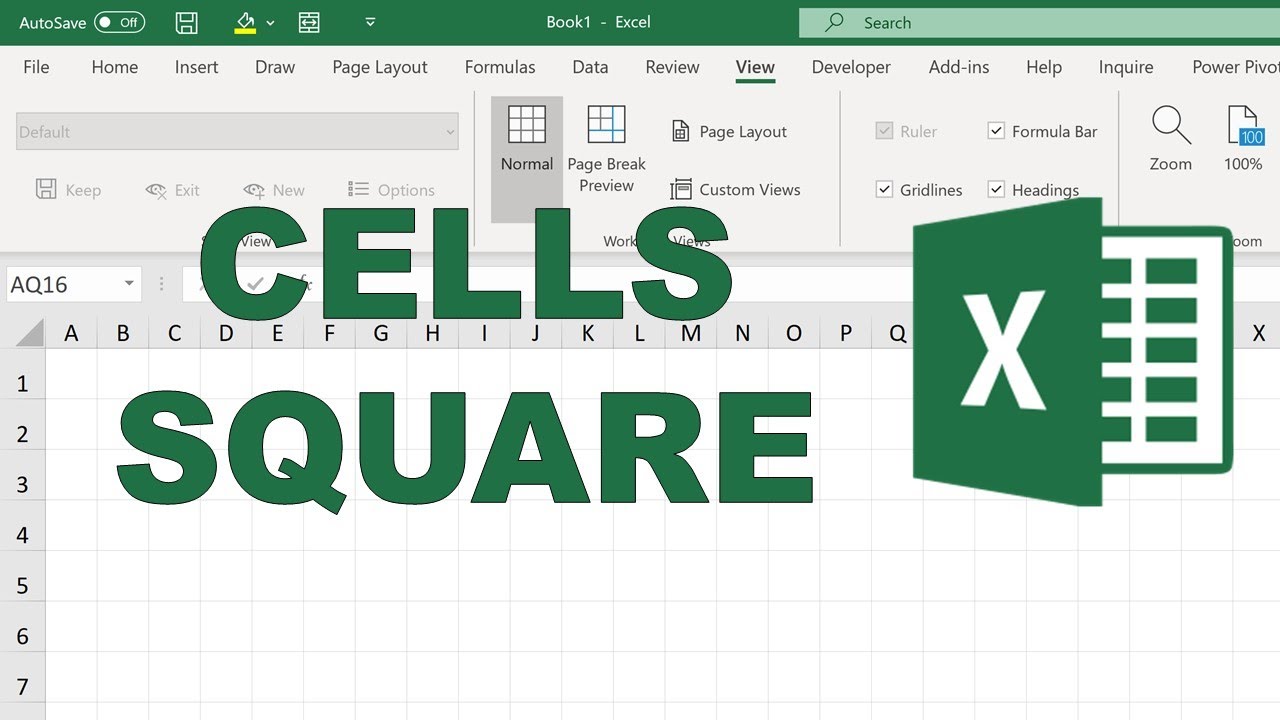
In Excel you can format square cells in two ways. In this practical tip you will learn which ways are open to you and how you can proceed.
First method: format square cells in Excel via the menu
The menu allows you to format the cells of an Excel table. With just a few clicks you can make sure that your cells are square.
- Select “Start” in the menu and mark the area of the table you want to format.
- If you want all cells of the table to be square, select the entire area by pressing [Ctrl] + [A].
- Find the area “Cells” in the ribbon and click on “Format”.
- Select “Cell height” first and then “Column width” to format the individual cells in height and width.
- However, you need to know which values result in square cells. This is the case, for example, with a cell height of 26.25 and a column width of 4.29.
Second method: Square cells in Excel with the mouse
Second option: format the cells in Excel with the mouse
- First select the area of the table you want to format. If you want to select everything, press [Ctrl] + [A].
- Now first drag the cells to the desired column width. To do this, place the mouse at the subdivision between column A and column B.
- Then do the same with the cell height. To do this, place the mouse pointer on the boundary between the first and second row. As soon as the current height is displayed, drag the boundary to the desired value while holding down the mouse button.
- If you select the same value for height and width, the cells are square.

