Index function in Excel – this is how it works

Excel offers an index function to call up data from tables and sub-tables. We explain how you can use this function

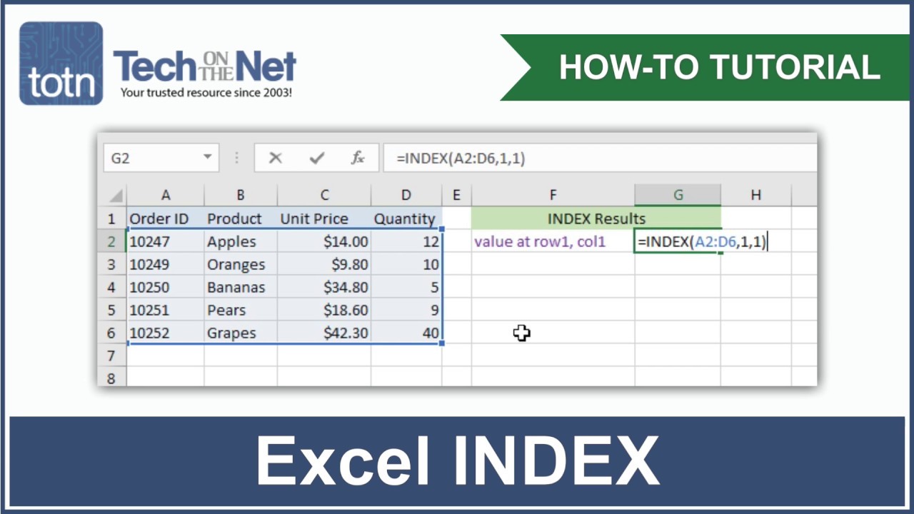
Using the index function in Excel

Excel is a spreadsheet calculation programme. You can call up individual entries in a table using the combination of row and column. You can create several sub-tables in a table. From these you can retrieve values with the index function. We will explain how this works with an example from Blumenhandel GbR.

• The flower trade GbR has an Excel document with the table “Statistics” and the sub-table “Working hours” (red).

• The list of employees forms the rows of the sub-table, a list of the days of the week forms the columns. The working hours per employee and day are entered (yellow).

• You can find out which employee worked how long on which day of the week with the index command: “=INDEX(Table;Row;Column)”, i.e. “=INDEX(Working hours;Employee list;Weekday list)”.

The comparison function

The index function is particularly useful in combination with the comparison function. This can relieve you of the task of counting the desired row and column.

• Enter the name of the desired employee in a cell. Alternatively, you can select the employee name using a drop-down menu.

• In another cell you can determine the row that corresponds to the row in the sub-table. To do this, enter “=VERGLEICH(Mitarbeiter;Mitarbeiterliste;0)”. The line number that corresponds to the name is output (yellow).

• Proceed in the same way with the weekday and column number (green).

• If you now use the index function, you can read in the numbers output by means of the comparison function (blue).