Inserting Harvey Balls in Excel

by Pramith October 13, 2026

written by Pramith October 13, 2026

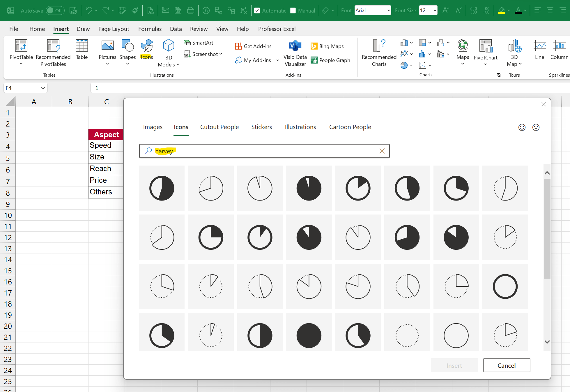
With Harvey Balls, you can also visualise percentages in Excel. We’ll show you how.

The following instructions were carried out using Excel 2013. In other versions, the individual options may be labelled or arranged differently.

Open Excel and use the mouse to select all the numbers (between 0 and 1) or percentages (between 0% and 100%) that you wish to convert into Harvey Balls.
Next, under the ‘Home’ tab, locate the ‘Formatting’ category.
Click the ‘Conditional Formatting’ button here and select the ‘Conditional Rule’ or ‘New Rule’ option.
Change the format style to ‘Icons’ and select ‘Five-Quart’ for the icon type.
You can now make a few personal adjustments. We recommend increasing the first value for the full circle from 80 to 100. This makes more sense in most cases.
In the “Type” column, you can choose between “Percentage” and “Number”, depending on the format of your source values.
The “Reverse symbol order” button means that 100&% is no longer displayed as a black circle, but as a white circle. Selecting “Show symbol only” hides the numbers associated with the Harvey Balls.
Click the “OK” button to insert the Harvey Balls into the Excel document.

Editing Harvey Balls in Excel

It’s rare that the Harvey Balls look just right on the first attempt. If you’d like to adjust the settings again, proceed as follows:

Select the desired cells in Excel again and click the ‘Conditional Formatting’ button at the top.
Select the ‘Manage Rules’ option and click the ‘Edit Rule’ button there.
If you’d like to display cells other than Harvey Balls, either add the cells to the relevant row or click the appropriate button next to the input field (see image).